Time Series Analysis
Time series analysis is useful for exploring a dataset which contains one or more time series. This kind of analysis allows you to perform statistical tests on time series, as well as to inspect some of its properties like the auto-correlation function.
All of these cards share common configuration options. In order to create or configure a time series analysis, you have to select a numerical (continuous) variable which holds the series values. You also have to select a time variable which holds the timestamps formatted according to the ISO8601 format.
If the dataset uses the long format to store the time series, it is possible to specify the time series identifiers by checking the corresponding checkbox. In this case, the variable name as well as the value used to discriminate the time series must be provided.
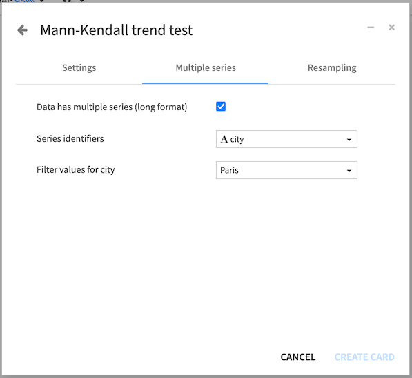
All time series card outputs include a summary for the time series, as well as the detected time step for the series.
Warning
Most of the time series computations require that the time series is evenly distributed with a constant time step. Resampling of a time series using a constant time step can be achieved by using the time series preparation plugin
The analysis cards are grouped into:
Stationarity and unit root tests
This kind of test allow you to assess whether a time series is stationary or has a unit root. A stationary series is a series which statistical properties do not change over time. Also, the presence of a unit root in a time series suggests that the series is not stationary.
By default, the number of lags that will be used by the test is automatically computed but you can choose to manually set this value if it suits your use case better.
The conclusion of a unit root test indicates whether the test rejects the hypothesis at the given significance level, or whether it is inconclusive.
Augmented Dickey-Fuller (ADF) test
The Augmented Dickey-Fuller test tests the hypothesis that there exists a unit root in the time series.

The configuration options allow to specify the regression model that is used by the test.
Zivot-Andrews test
The Zivot-Andrews test tests the hypothesis that there exists a unit root with one structural break in the time series.

The configuration options allow to specify the regression model that is used by the test.
Kwiatkowski-Phillips-Schmidt-Shin (KPSS) test
The KPSS test tests the hypothesis that the time series is stationary.

The configuration options allow to specify the regression model that is used by the test.
Trend
This kind of analysis allows to inspect the trend of a time series.
STL decomposition plot
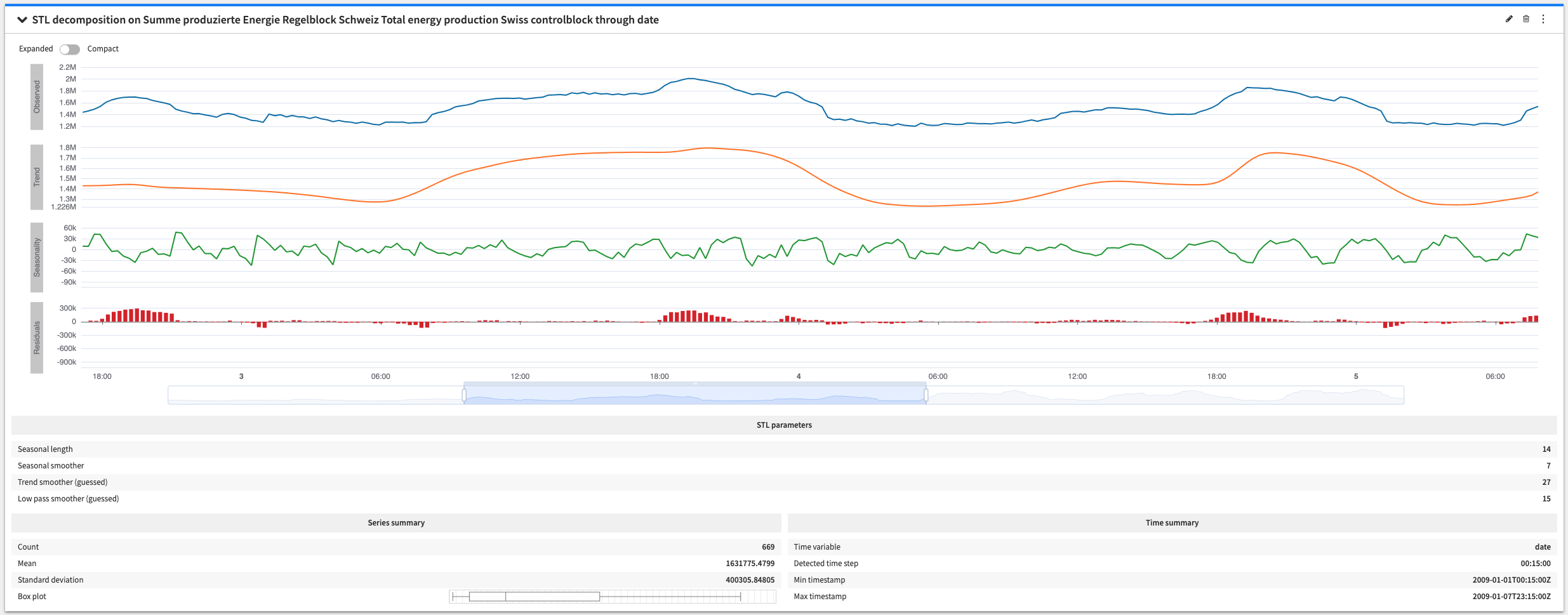
The STL decomposition plot is used to visualize the trend and seasonality of a series.
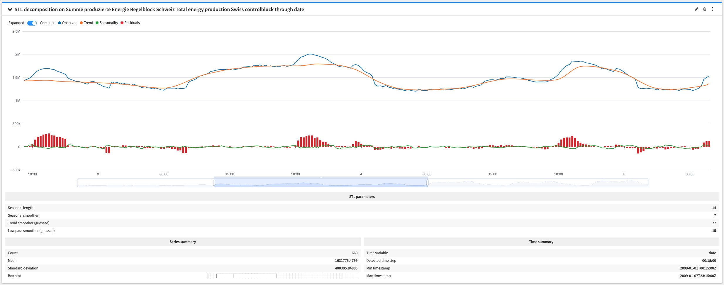
You can also enable the compact view to display the original series and its components (trend, seasonality and residuals) on a uniform scale. This not only makes comparing series with similar scales easier (usually the original series and the trend series), but also helps identifying differences in scale among the series.
The configuration options give control over the type of decomposition that you want (additive or multiplicative) and over the STL decomposition algorithm parameters.
Note
The parameters of the STL decomposition algorithm are the ones from the statsmodels library. For more information visit the statsmodels documentation.
Mann-Kendall trend test
The Mann-Kendall trend Test is used to analyze series data for consistently increasing or decreasing trends (monotonic trends). It tests the hypothesis that there is no monotonic trend in the time series.
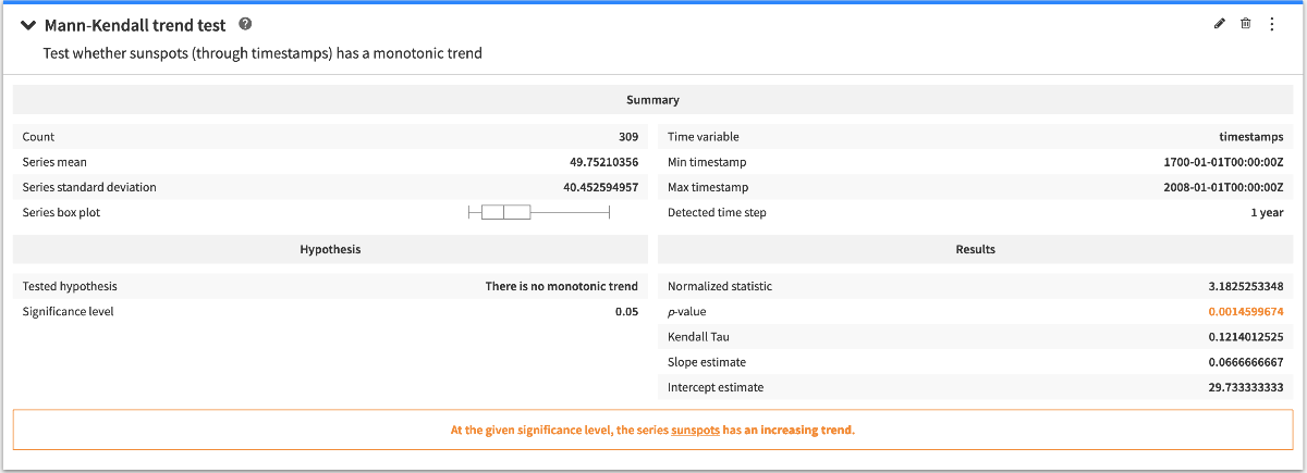
The conclusion of the Mann-Kendall trend test indicates whether the test rejects the hypothesis at the given significance level, or whether it is inconclusive.
Auto-correlation
The auto-correlation analyses allow to inspect the degree of correlation of a time series with lagged versions of itself (with a given number of lags).
Auto-correlation function plot
The auto-correlation function plot allows to visually inspect the auto-correlation function of a time series. For each lag and coefficient, the confidence interval is displayed in the background.
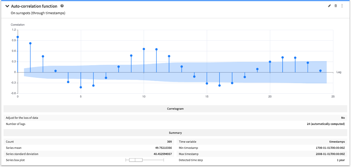
The configuration options give control on whether the coefficients must be adjusted to account for the loss of data.
By default, the number of lags that will be used to compute the coefficients is automatically computed but you can choose to manually set this value if it suits your use case better.
Note
The configuration options allows to quickly jump between auto-correlation and auto-correlation functions.
Partial auto-correlation function plot
The partial auto-correlation function plot allows to visually inspect the partial auto-correlation function of a time series. For each lag and coefficient, the confidence interval is displayed in the background.
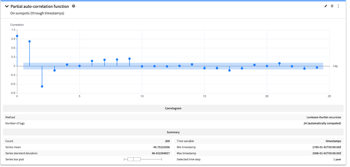
The configuration options allow to specify the method to use for computing the coefficients.
By default, the number of lags that will be used to compute the coefficients is automatically computed but you can choose to manually set this value if it suits your use case better.
Note
The configuration options allows to quickly jump between auto-correlation and auto-correlation functions.
Durbin-Watson statistic
The Durbin-Watson statistic gives a measurement for the first order auto-correlation of a time series (with a lag value of 1). The statistical test associated to this statistic tests the hypothesis that there is no first order auto-correlation in the time series.

The conclusion of the Durbin-Watson statistic analysis tells whether the statistic shows evidence of positive or negative auto-correlation.
