Time Series Forecasting Results

When a model finishes training, click on the model to see the results.

Forecast charts

The model report contains a visualization of the time series forecast vs. the ground truth of the target variable. If quantiles were specified, this graph also contains the forecast intervals.

If K-Fold cross-test is used for evaluation, the forecast and forecast intervals are shown for every fold.

For multiple time series datasets, one visualization per time series is provided.

Explainability: Feature importance

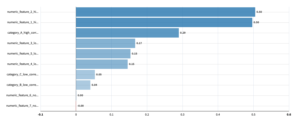
Permutation feature importance measures how much the model prediction error (MASE) increases when the values of a given feature are randomly shuffled.

A positive importance means the feature contributes to model accuracy: when shuffled, prediction error increases.

A negative importance suggests removing the feature could improve accuracy.

For models trained with external features, Dataiku can compute permutation feature importance and rank the top 20 features by their impact on the model prediction error (MASE).

The importance values are computed over the entire historical dataset, with a score performed on the first horizon of the test set. The computation can be slow for datasets with many features, or many time series identifiers.

Note

By default, feature importance computation is skipped during training and can be computed on-demand from the model report. Uncheck “Skip Feature importance” (Design > Runtime environment > Performance tuning) to compute feature importance during training.

Global feature importance

Global feature importance shows the aggregated impact of features across all time series.

Per time series feature importance

For datasets with multiple time series, Dataiku can compute feature importance for each individual time series. This helps identify features that work differently across different series.

Warning

Per-identifier computation can be significantly more time-consuming.

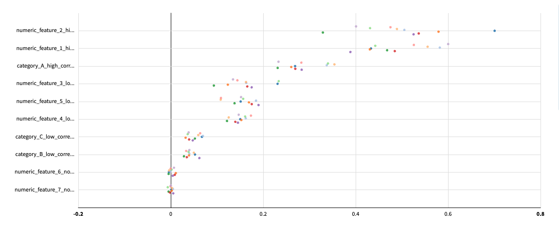
Each dot represents the importance of a feature for a specific time series. You can filter the displayed time series using the identifier dropdown menus.

Note

When enabling feature importance during training, you can check “Calculate per-identifier feature importance” to instead compute this more detailed analysis.

Note

When many time series are present, only the first 100 are loaded by default.

Limitations

Only external features are included in the permutation importance, the target is excluded.

Availability

Feature importance is only available for models using numerical or categorical external features.

It is not available in the following cases:

• Models without external features

• Models using text features

Performance: Metrics

For multiple time series datasets, metrics are aggregated over all time series.

If at least one time series has an undefined metric, then the aggregated metric is also undefined.

If K-Fold cross-test is used for evaluation, these aggregated metrics are then averaged over all folds, ignoring folds that yield undefined metric values.

Time series aggregation methods by metric

Metric	Aggregation method
Mean Absolute Scaled Error (MASE)	Average across all time series
Mean Absolute Percentage Error (MAPE)	Average across all time series
Symmetric MAPE	Average across all time series
Mean Absolute Error (MAE)	Average across all time series
Mean Squared Error (MSE)	Average across all time series
Mean Scaled Interval Score (MSIS)	Average across all time series
Mean Absolute Quantile Loss (MAQL)	First compute the mean of each quantile loss across time series then compute the mean across all quantiles
Mean Weighted Quantile Loss (MWQL)	First compute the mean of each quantile loss across time series then compute the mean across all quantiles. Finally divide by the sum of the absolute target value across all time series
Root Mean Squared Error (RMSE)	Square-root of the aggregated Mean Squared Error (MSE)
Normalized Deviation (ND)	Sum of the absolute error across all time series, divided by the sum of the absolute target value across all time series

Performance: Per time series metrics

For multiple time series datasets, DSS also shows the metrics of each individual time series.

If K-Fold cross-test is used for evaluation, per time series metrics are aggregated over each fold for each time series, ignoring folds that yield undefined metric values.

Model Information: Algorithm

For multiple time series datasets, some models train one algorithm per time series under the hood (mainly ARIMA and Seasonal LOESS). The resulting per times series hyperparameters are shown in this tab, if any.

Model Information: Model Coefficients

Some models, such as ARIMA, ETS, Prophet, etc. have a set of coefficients that can be used to interpret the model. Those coefficients are shown in this tab. When applicable, the p-values and t-values of those coefficients can also be shown.

Model Information: Residuals

Residuals are differences between observed data points and the values predicted by the model. Analysis of such residuals is useful to assess how a model behaves on the historical data it has been optimized on. In Dataiku, those residuals can be visualized with 4 graphs.

Note

Residuals are computed for every possible value of the historical data. Therefore their computation can take a long time. The computation can be manually skipped by checking “Skip expensive reports” before training the model (Design > Runtime environment > Performance tuning).

Standardized residuals histogram

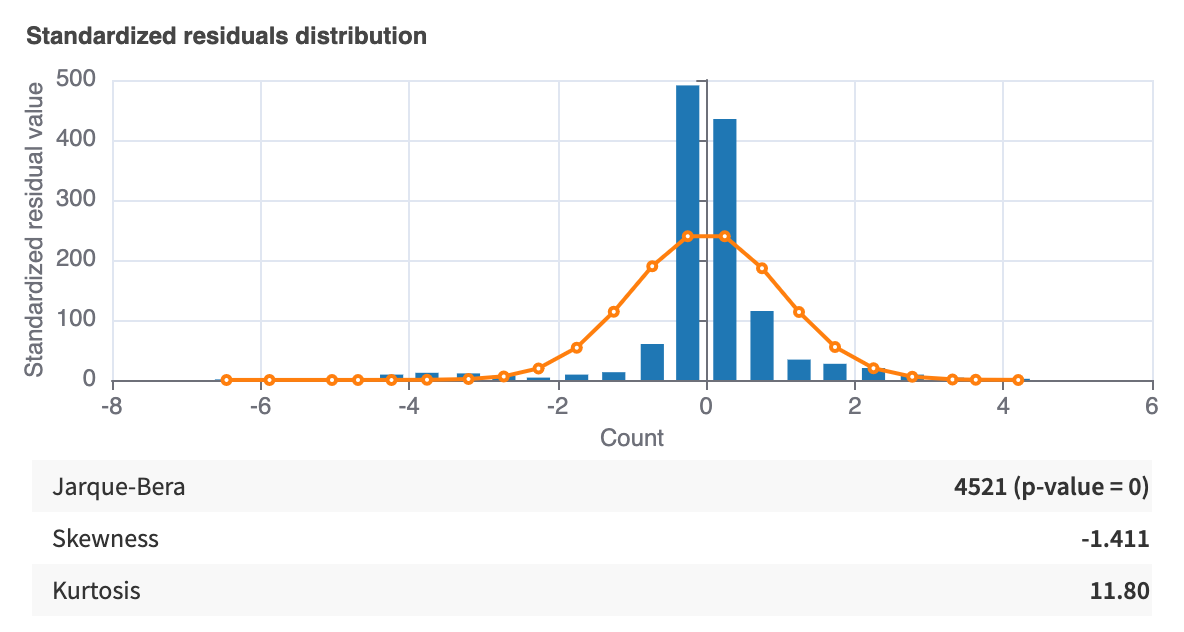
This graph represents the distribution of standardized residuals. Alongside the histogram is plotted a z-distribution.

Standardized residuals over time

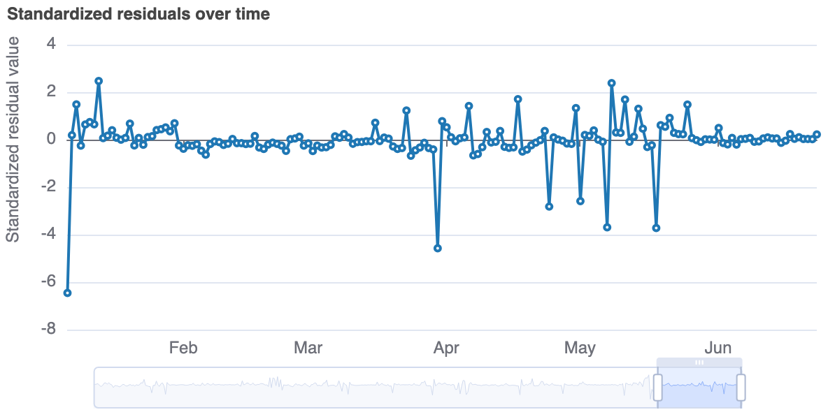
This plot is a representation of the standardized residuals over time. In simpler terms, this is a standardized representation of the error on the historical data.

Normal Q-Q Plot

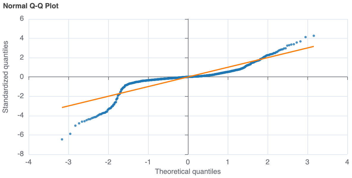
A Q-Q plot is a plot of standardized residuals against what would be a theoretical z-distribution of residuals.

Correlogram

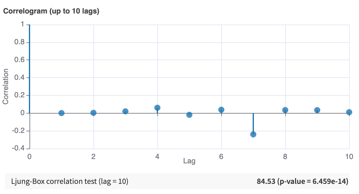
This is a plot of auto-correlation computed for different lag values (up to 10).

Model Information: Information criteria

Information criteria, such as the Akaike Information Criterion (AIC), Bayesian Information Criterion (BIC), and Hannan-Quinn Information Criterion (HQIC), are metrics that help in model selection by evaluating the trade-off between a model’s goodness of fit and its complexity.

Use these criteria to compare different models trained on the same dataset. A model with a lower information criterion value is generally preferred, as it indicates a better balance between accuracy and simplicity, which can help prevent overfitting.

Note

These criteria are only available for statistical models (ARIMA, ETS, Seasonal Trend) where a likelihood function can be calculated.