Advanced models optimization
Each machine learning algorithm has some settings, called hyperparameters.
For each algorithm that you select in DSS, you can ask DSS to explore several values for each hyperparameter. For example, for a regression algorithm, you can try several values of the regularization parameter. If you ask DSS to explore several values for hyperparameters, all the combination of values will be assessed in a “hyperparameter optimization” phase.
Instead of searching for specific discrete values, like “1, 3, 10, 30”, DSS can also search for hyperparameters in continuous ranges like “between 1 and 30”.
DSS will automatically train a model for each combination of hyperparameters and keep the one that maximizes the metric chosen in the Metric section. To do so, DSS splits the train set and extracts a hold-out set (or cross-validation set). Each combination of hyperparameters is then evaluated by training a model on the train set minus the hold-out set and evaluating it on the hold-out set. When the evaluation is performed on a partition of the train set in k subsets of equal size, each acting successively as the hold-out, this method is called K-Fold cross-validation.
Note
During this optimization of hyperparameters, DSS never uses the test set (see Train / Test), which must remain “pristine” for the final evaluation of the model quality.
Hyperparameter points that yield undefined metric values (NaN or infinity) are ignored during the search.
DSS gives you a lot of settings to tune how the search for the best hyperparameters is performed.
Search strategies
Grid search
The most classical strategy for optimizing search parameters is called “Grid search”. For each hyperparameter, you specify either a list of values to test, or a range specification like “5 values equally spaced between 30 and 80” or “8 values logarithmically spaced between 1 and 1000”.
DSS tries all combinations of all hyperparameters as discrete “grid points”.
The grid can either be explored in order or in a shuffled order. Shuffling the grid tends to find better points earlier on average, which is preferable if you want to interrupt search.
Random search
Instead of exploring discrete points on a grid, random searching considers hyperparameters as a continuous spaces and tests randomly-chosen points in the hyperparameters space.
For each hyperparameter, you specify a range to test. DSS will then pick random points in the space defined by all parameters and test them.
A Random search is by nature infinite, so it is mandatory to select a maximum number of iterations and/or maximum time before stopping the search.
Bayesian search
Bayesian search starts like a Random search, but as new points in the hyperparameters space are tried, a predictive model is trained in order to model the search space. This predictive model is used to refine the search in order to focus on the most promising parts of the hyperparameters search, in order to reach a good set of hyperparameters faster.
DSS bayesian search leverages a dedicated python package, scikit-optimize, and therefore requires to run on a code-env, with the appropriate packages installed. To do so, you need to:
Create a new code environment
Go to the “Packages to install” tab of this code-env and click on “Add sets of packages”
Select one of the package presets containing scikit-optimize (e.g. “Visual Machine Learning and Visual Time series forecasting (CPU)”) and click “Add”
Update your code-env
You can now select the code-env in the “Runtime environment” tab of the Design part of the Lab, and train your experiments leveraging bayesian search.
Cross-validation
There are several strategies for selecting the cross-validation set.
Simple split cross-validation
With this method, the training set is split into a “real training” and a “cross-validation” set. The split is performed either randomly, or according to a time variable if “Time-based ordering” is activated in the “Train/test split” section. For each value of each hyperparameter, DSS trains the model and computes the evaluation metric, keeping the value of the hyperparameter that provides the best evaluation metric.
The obvious drawback of this method is that restricts further the size of the data on which DSS truly trains. Also, this method comes with some uncertainty, linked to the characteristics of the random split.
K-Fold cross-validation
With this method, by default the training set is randomly split into K equally sized portions, known as folds.
For each combination of hyperparameter and each fold, DSS trains the model on K-1 folds and computes the evaluation metric on the last one. For each combination, DSS then computes the average metric across all folds. DSS keeps the hyperparameter combination that maximizes this average evaluation metric across folds and then retrains the model with this hyperparameter combination on the whole training set.
Note that if “Time-based ordering” is activated in the “Train/test split” section, the training set is split into K equally sized portions sorted according to the time variable, and the training splits are assembled in order to ignore samples posterior to each evaluation split so as to emulate a forecasting situation (see e.g. https://scikit-learn.org/stable/modules/generated/sklearn.model_selection.TimeSeriesSplit.html)
This method increases the training time (roughly by K) but allows to train on the whole training set (and also decreases the uncertainty since it provides several values for the metric).
Note
The methodology for K-Fold cross-validation is the same as K-Fold cross-test but they serve different goals. K-Fold cross-validation aims at finding the best hyperparameter combination. K-Fold cross-test aims at evaluating error margins on the final scores by using the test set.
Using K-Fold for both cross-test and cross-validation
When using K-fold strategy both for hyperparameter search (cross-validation) and for testing (cross-test), the following steps are applied for all algorithms:
Hyperparameter search: The dataset is split into K_val folds. For each combination of hyperparameter, a model is trained K_val times to find the best combination. Finally, the model with the best combination is retrained on the entire dataset. This will be the model used for deployment.
Test: The dataset is split again into K_test folds, independently from the previous step. The model with the best hyperparameter combination of Step 1 is trained and evaluated on the new test folds. The performance metric is reported as the average across test folds, with min-max values for estimating uncertainty.
The two steps are done independently, but are shared for all algorithms. Hence one algorithm is compared to another using the same folds.
The number of model trainings needed for a given algorithm to go through the two steps is:
Stratified & Grouped K-Fold
Folds can be stratified with respect to the prediction target, so that the percentage of samples for each class is preserved in each fold. This is applicable only for classification tasks.
Folds can also be grouped. The training set is then split according to the values of the selected “group column”. This means that all rows from the same group go into the same fold (but if K is less than the number of groups, multiple groups can share the same fold). You cannot have fewer groups than folds.
Stratified group k-fold is possible, in which case the stratification is best-effort: the folds are stratified as far as possible, while always maintaining the groups.
Note
For stratified group k-fold, the split is not shuffled and ignores the random seed parameter, to avoid a bug in scikit-learn leading to incorrect stratification when shuffled.
The main difference between grouped + stratified and grouped-only k-fold is:
Group k-fold attempts to balance the folds by keeping the number of distinct groups approximately the same in each fold.
Stratified group k-fold attempts to balance the folds by keeping the target distribution approximately the same in each fold.
Custom
Note
This only applies to the “Python in-memory” training engine
If you are using scikit-learn, LightGBM or XGBoost, you can provide a custom cross-validation object. This object must follow the protocol for cross-validation objects of scikit-Learn.
See: http://scikit-learn.org/stable/modules/cross_validation.html
Retrieving column names in the custom cross validator
In order to have access to the column names of the preprocessed dataset, a method called set_column_labels(self, column_labels) can be implemented in the CV object.
If this method exists, DSS will automatically call it and provide the list of the column names as argument.
Warning
The column labels passed to the function set_column_labels are the labels of the prepared and preprocessed columns resulting from the preparation script followed by features handling. Hence, their name may not correspond to the original columns of the dataset.
For instance, if automatic pairwise linear combinations were enabled, some columns may take the form: pw_linear:<A>+<B>. To find the exact name of the columns, it is advisable to print the column labels received in set_column_labels.
Example
Warning
Classes cannot be declared directly in the Models > Design tab. They should be packaged in a library and imported, as demonstrated in the examples below.
In the “Custom Cross-validation strategy” code editor, you should create the
cvvariable.from my_custom_cv import MyCustomCV cv = MyCustomCV()
In a library file called
my_custom_cv.py:class MyCustomCV(object): def set_column_labels(self, column_labels): self.column_labels = column_labels def _extract_important_column(self, X): # The two following instructions show how to retrieve a specific # column given its name # 1. Retrieve the index of the column called "important_column" column_index = self.column_labels.index("important_column") # 2. Retrieve the corresponding data column return X[:, column_index] def split(self, X, y, groups=None): important_column = self._extract_important_column(X) # Finish the implementation of the split function ... def get_n_splits(self, X, y, groups=None): important_column = self._extract_important_column(X) # Finish the implementation of the get_n_splits function ...
Execution parameters
Each algorithm is trained in isolation from the other algorithms but they all use the same execution parameters for their own hyperparameter search.
You can select the maximum number of algorithms trained concurrently in the Advanced > Runtime environment design screen (“Max concurrency” setting).
Limits
You can specify two types of limits to the hyperparameter search execution:
hyperparameter space: each algorithm will explore at most the specified number of hyperparameter combinations
search time: for each algorithm, the search will stop when the time limit is reached.
For grid-search, the hyperparameter space is naturally limited so specifying any limit is optional.
For random or Bayesian search, the hyperparameter space is usually unlimited so specifying at least one of these limitations is mandatory.
Note that when both space and time limits are set, the one to be enforced is the first to be reached.
Distribution and multi-threading
Distribution: since version 9.0, you can leverage a Kubernetes cluster to distribute and speed up the hyperparameter search. You can specify a number of containers where the preprocessed train data will be sent to, and where the training and evaluation of the model for all splits and hyperparameters combinations will be performed. As a result, the search can be sped up by a factor of up to the number of containers.
Note that the “Containerized execution configuration” setting in Advanced > Runtime environment needs to be specified with a configuration using a Kubernetes engine for this option to be available.
Number of threads: Dataiku can also speed up the search by using multi-threading in the exploration of the different combinations of data splits and hyperparameters. More specifically, each thread will be used to explore sequentially the different splits and hyperparameters combinations. When containerized execution is used, this setting controls the number of threads in each container. Note that using many threads may increases memory usage. Note also that significant speedups can only be expected for algorithms releasing the Python GIL during training, such as e.g. tree-based scikit-learn algorithms.
Randomization
The order in which hyperparameters are drawn can be controlled through the “Random state” setting. It guarantees reproducibility of the hyperparameter search, provided that all other randomness factors are kept identical.
For grid-search, you can specify whether or not the grid is explored in the natural order. Shuffling can speed up the search by removing priority between hyperparameters, avoiding thorough explorations of hyperparameters with low impact on the result.
Interrupting and resuming hyperparameter search
If you select a large number of hyperparameters to optimize and hyperparameter values, training can become very slow.
Interrupting
At any time while DSS is searching, you can choose to interrupt the optimization. DSS will finish the current point it is evaluating, and will train and evaluate the model on the “best hyperparameters found so far”.
If you are using Grid search strategy, we recommend that you enable “Randomize grid search” if you plan on interrupting your grid search.
Time-bounding or iteration-bounding
Alternatively, before starting the search, you can select a maximum time or number of points to evaluate. DSS will automatically interrupt the search when one of these criteria is reached.
Resuming
An interrupted hyperparameter search can be resumed later on. DSS will only try the hyperparameter values that it hadn’t tried yet.
Visualization of hyperparameter search results
If you have selected several hyperparameters for DSS to test, during training, DSS will show a graph of the evolution of the best cross-validation scores found so far. DSS only shows the best score found so far, so the graph will show “ever-improving” results, even though the latest evaluated model might not be good. If you hover over one of the points, you’ll see the evolution of hyperparameter values that yielded an improvement.
In the right part of the charts, you see final test scores for completed models (models for which the hyperparameter-search phase is done)
The timing that you see as X axis represents time spent training this particular algorithm. DSS does not train all algorithms at once, but each algorithm will have a 0-starting X axis.
Note
The scores that you are seeing in the left part of the chart are cross-validation scores on the cross-validation set. They cannot be directly compared to the test scores that you see in the right part.
They are not computed on the same data set
They are not computed with the same model (after hyperparameter-search, DSS retrains the model on the whole train set)
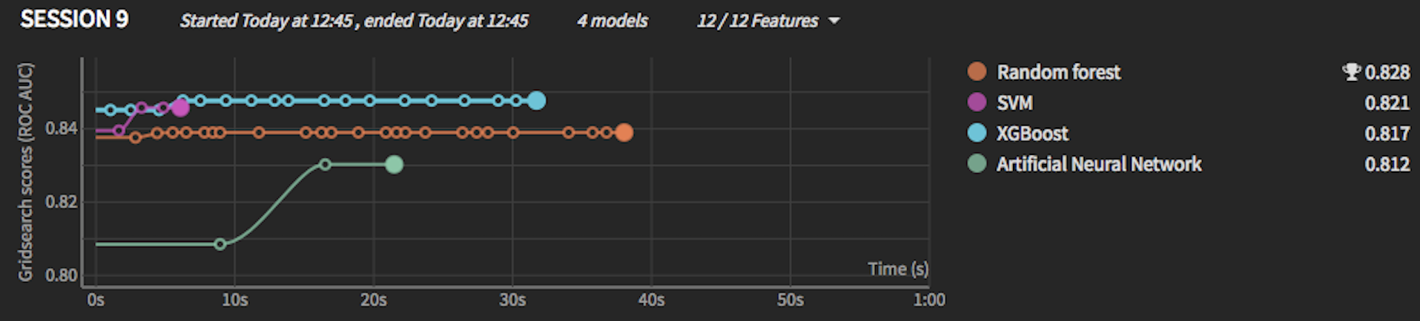
In this example:
Even though XGBoost was better than Random Forest in the cross-validation set, ultimately on the test set (once trained on the whole dataset), Random forest won (this might indicate that the RF didn’t have enough data once the cross-validation set was out)
The ANN scored 0.83 on the cross-validation set, but its final score on the test set was slightly lower at 0.812
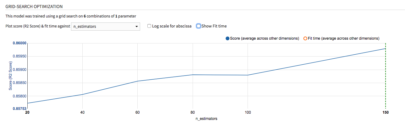
In a model
Once a model is done training, you can also view the impact of each individual hyperparameter value on the final score and training time. This information is displayed both as a graph and a data table that you can export.