
Individual prediction explanations
Dataiku DSS provides the capability to compute individual explanations of predictions for all Visual ML models that are trained using the Python backend (this includes custom models and algorithms from plugins, but not Keras/Tensorflow models).
The explanations are useful for understanding the prediction of an individual row and how certain features impact it. A proportion of the difference between the row’s prediction and the average prediction can be attributed to a given feature, using its explanation value. In other words, you can think of an individual explanation as a set of feature importance values that are specific to a given prediction.
DSS provides two modes for using the individual prediction explanations feature:
In the model results page, to visualize the explanations.
With the scoring recipe, to return the explanation values along with the predictions.
In the model results
The Individual explanations tab in the results page of a model is an interactive interface for providing a better understanding of the model.
As an example, consider the case where the global feature importance values for a black-box model may not be enough to understand its internal workings. In such a situation, you can use this mode to compute the explanations for extreme predictions (i.e. for records that output low and high predictions) and to display the contributions of the most influential features. You can then decide whether these features are useful from a business perspective.
For speed, DSS uses different samples of the dataset to compute explanations, depending on the splitting mechanism that was used during the model design phase.
If the model was built on training data (using a train/test split), DSS computes the explanations on a sample of the test set.
If cross-validation was used during the model design phase, then DSS computes the explanations on a sample of the whole dataset.
You can modify settings for the sample by clicking the gear icon in the top right of the individual explanations page. The interactive interface also allows you to specify values for other parameters, such as:
The number of highly influential features to explain (or desired number of explanations).
The method to use for computing explanations.
An approximate number of records of interest at the low and high ends of the predicted probabilities.
A column to use for identifying the explanations of each record.
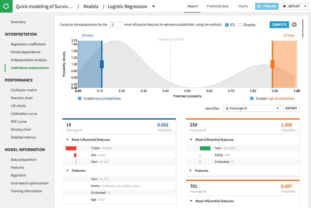
The result of the computation is a list of cards, one card per prediction. The cards on the left side of the page are for the records that give low predictions, while those on the right side of the page are for high predictions. Within the cards, bars appear next to the most influential features to reflect the explanation values. Green bars oriented to the right reflect positive impacts on the prediction, while red bars oriented to the left reflect negative impacts.
Note
If the model was trained in a container, then this computation will be implemented in a container. Otherwise, the computation will be implemented on the DSS server. The same is true for other post-training computations like partial dependence plots and subpopulation analysis.
With the scoring recipe
The individual prediction explanations feature is also available within a scoring recipe (after deploying a model to the flow).
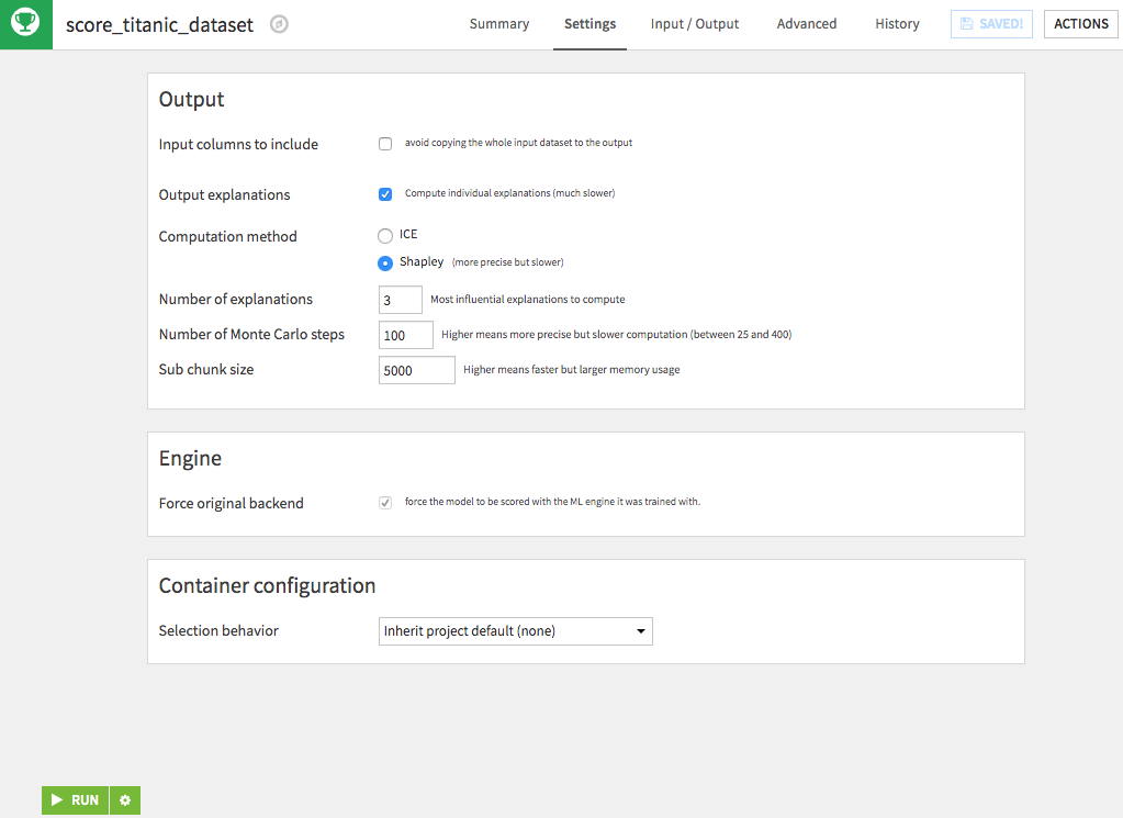
If your model is compatible, i.e. a Visual ML model that is trained using the Python backend (this includes custom models and algorithms from plugins, but not Keras/Tensorflow models), then the option for Output explanations is available during scoring. Activating this option allows you to specify the number of highly influential features to explain, and to select the computation method. It also forces the scoring to use the original Python backend.
Note
By default, the scoring recipe is performed in memory. However, you can choose to perform the execution in a container.
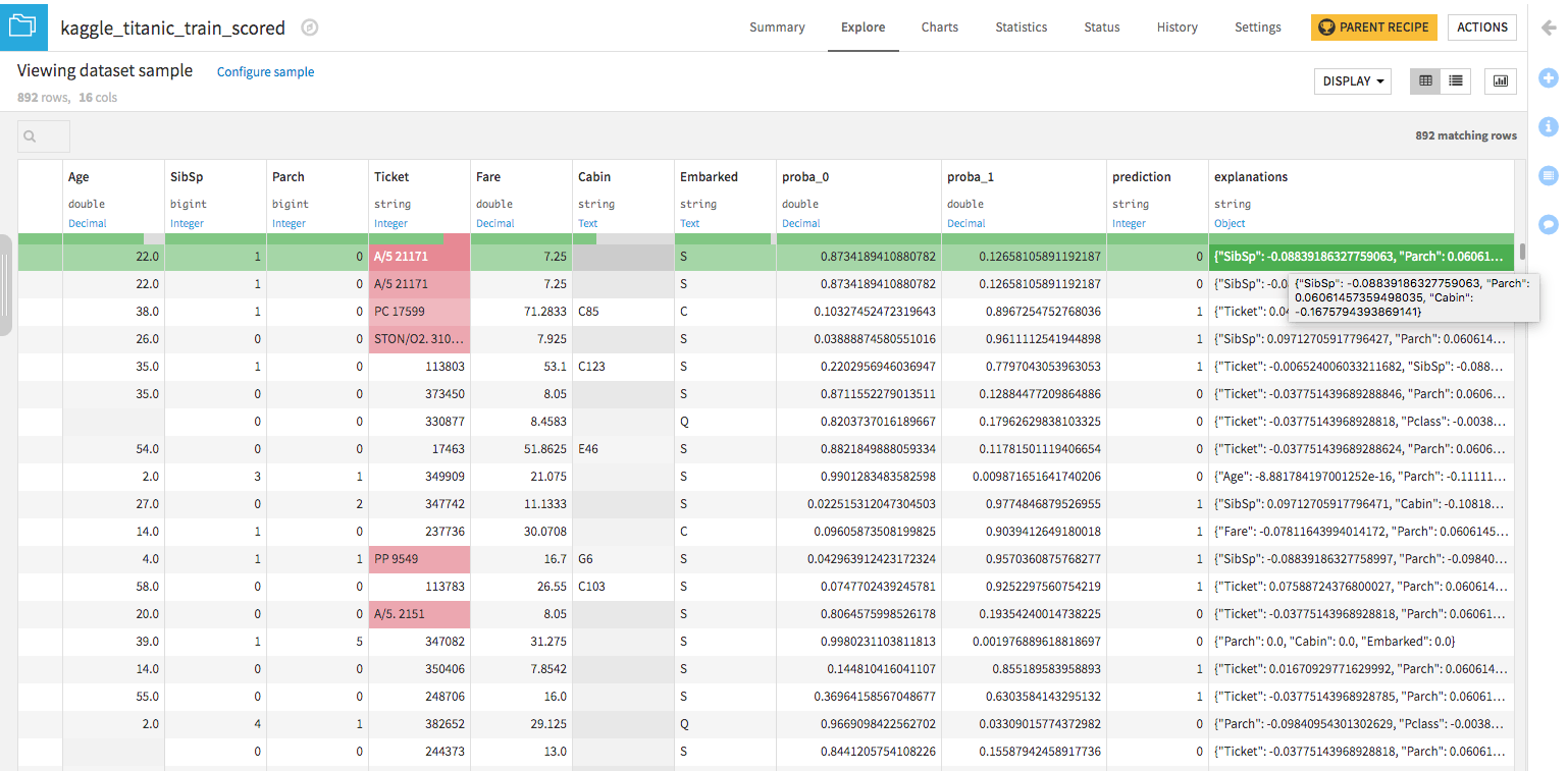
Running the scoring recipe outputs the predictions and an explanations column. The explanations column contains a JSON object with features as keys and computed influences as values, and can easily be unnested in a subsequent preparation recipe.
Computation methods
To compute the individual prediction explanations, DSS provides two methods based on:
The Shapley values
The Individual Conditional Expectation (ICE)
Method 1: Based on the Shapley values
This method estimates the average impact on the prediction of switching a feature value from the value it takes in a random sample to the value it takes in the sample to be explained, while a random number of feature values have already been switched in the same way.
To understand how the method based on Shapley values works, consider that you have a data sample \(X\), and you want to explain the impact of one of its features \(i\) on the output prediction \(y\). This method implements these main steps:
Create a data sample \(X^\prime\) by selecting a random sample from your dataset and switching a random selection of its features (excluding the feature of interest \(i\)) to their corresponding values in \(X\). Then compute the prediction \(y^\prime\) for \(X^\prime\).
Switch the value of the feature \(i\) in \(X^\prime\) to the corresponding value in \(X\), to create the modified sample \(X^{\prime\prime}\). Then compute its prediction \(y^{\prime\prime}\).
Repeat the previous steps multiple times, and average the predictions \(y^{\prime\prime}\), to determine an average prediction.
Finally, compute the difference between the average prediction and \(y^\prime\) to obtain the impact that feature \(i\) has on the prediction of \(X\).
The number of random samples used in the implementation depends on the expected precision and the non-linearity of the model. As a guideline, multiplying the number of samples by four improves the precision by a factor of two. Also, a highly non-linear model may require 10 times more samples to achieve the same precision of a linear model. Because of these factors, the required number of random samples may range from 25 to 1000.
Finally, the overall computation time is proportional to the number of highly influential features to be explained and the number of random samples to be scored.
Method 2: Based on ICE
This method explains the impact of a feature on an output prediction by computing the difference between the prediction and the average of predictions obtained from switching the feature value randomly. This method is a simplification of the Shapley-value-based method.
To understand how the method based on ICE works, consider that you have a data sample \(X\), and you want to explain the impact of one of its features \(i\) on the output prediction \(y\). This method implements these main steps:
Switch the value of the feature \(i\) in \(X\) to a value chosen randomly. Then compute its prediction \(y^\prime\).
Repeat the previous step multiple times, and average the predictions \(y^\prime\), to determine an average prediction.
Finally, compute the difference between the average prediction and \(y\) to obtain the impact that the feature \(i\) has on the prediction of \(X\).
For binary classification, DSS computes the explanations on the logit of the probability (not on the probability itself), while for multiclass classification, the explanations are computed for the class with the highest prediction probability.
More about the computation methods
The ICE-based method is faster to implement than the Shapley-based method. When ICE is used with scoring, the computation time (about 20 to 50 times longer than with simple scoring) is faster than that for the method based on Shapley values.
A major drawback of using the ICE-based method is that the sum of explanations over all the feature values is not equal to the difference between the prediction and the average prediction. This discrepancy can result in a distortion of the explanations for models that are non-linear.
The performance of the ICE-based method is model-dependent. Therefore, when choosing a computation method, consider comparing the explanations from both methods on the test dataset. You can then use the ICE-based method (for speed) if you are satisfied with its approximation.
For more details on the implementation of these methods in DSS, see this document.
Limitations
The computation for individual prediction explanations can be time-consuming. For example, to compute explanations for the five most influential features, expect a computation time multiplied by a factor of 10 to 1000, compared to simple scoring. This factor also depends on the characteristics of the features and of the computation method used.
For a given prediction, individual explanations approximate the contribution of each feature to the difference between the prediction and the average prediction. When that difference is small, the computation must be done with more random samples, to account for random noise and to return meaningful explanations.
When the number of highly influential features to be explained is fewer than the number of features in the dataset, it is possible to miss an important feature’s explanation. This can happen if the feature has a low global feature importance, that is, the feature may be important only for a small fraction of the samples in the dataset.
Individual prediction explanations are available only for Visual ML models that are trained using the Python backend (this includes custom models and algorithms from plugins, but not Keras/Tensorflow or computer vision models).
Using the Scoring Recipe with individual explanations can be very memory consuming. You can tweak the Scoring Recipe parameters to decrease the memory footprint. However, this will slow down the run. In particular:
If you are using “Shapley” method, the “Sub chunk size” and “Number of Monte Carlo steps”. Decreasing “Sub chunk size” should have the biggest impact
In “Advanced” tab, the “Python batch size”