
Generate features
The “generate features” recipe makes it easy to enrich a dataset with new columns in order to improve the results of machine learning and analytics projects.
DSS will then automatically join, transform, and aggregate this data, ultimately creating new features.
You can also configure time settings to avoid prediction leakage or specify more narrow time windows for computations.
Create a generate features recipe
Either select a dataset and click on the “Generate features” icon in the right panel, or click on the “+Recipe” button and select Visual > Generate features.
The recipe input should be your primary dataset, i.e. the dataset to enrich with new features.
Create your output dataset. It should be on the same connection as the primary dataset.
Note
The generate features recipe only supports datasets that are compatible with Spark or with SQL views. Connections compatible with SQL views include:
PostgreSQL
MySQL
Oracle
SQL Server
Azure Synapse
Vertica
Greenplum
DB2
Redshift
Snowflake
BigQuery
Teradata
Exasol
Databricks
Trino/Starbust
Set up data relationships
In the “Data relationships” section, you can add enrichment datasets and configure associated data relationships and join conditions. You may also specify time settings to avoid prediction leakage or add time windows.
Set up relationships without time settings
If you are not familiar with the recipe or if your primary dataset does not have a notion of time, follow these steps to add new relationships to enrich your primary dataset.
After creating a recipe with a primary dataset, click on “Add enrichment dataset”
Set the cutoff time to “None”
Add an enrichment dataset, and hit save
If you want to edit the auto-selected join conditions, click on them from the recipe window. If no join conditions have been auto-selected, click “add a condition” and add join keys.
Based on the join conditions, select the relationship type between your datasets. This will determine whether new features are generated from one or many rows. Select :
One-to-one if one row in the left dataset matches one row in the right dataset. Only row-by-row computations will be performed.
Many-to-one if many rows in the left dataset match one row in the right dataset. Only row-by-row computations will be performed.
One-to-many if one row in the left dataset matches several rows in the right dataset. Both row-by-row computations and aggregations will be performed.
Note
If the relationship type is one-to-many, the join key(s) will be used as the group key(s) when computing many-row aggregation features.
To add more than one enrichment dataset, click the “+” button next to the dataset you want to join onto.
The relationship type has a significant impact on the computations:
If the relationship type is one-to-one or many-to-one, the recipe will:
Perform a left join between the two datasets
Perform selected row-by-row computations
If the relationship type is one-to-many, the recipe will:
Group the right dataset by the join key(s) & perform selected aggregations
Perform a left join between the two datasets
Perform selected row-by-row computations
Build relationships with time settings
Defining time settings allows you to avoid data leakage in your new features, or to narrow the range of time used in feature generation. This involves a few key concepts :
Cutoff time: A date column in the primary dataset that indicates the point in time at which data from enrichment datasets should no longer be used in feature generation. This is a required step before adding time settings to enrichment datasets. For many use cases, the cutoff time is the time at which predictions should be made. For prediction problems, the notion of cutoff time is similar to the concept of time variable or time ordering.
Time index: Column from an enrichment dataset indicating when an event, corresponding to each row of data, occurred. If you set a time index in an enrichment dataset, all rows from the enrichment dataset whose time index value is greater than or equal to the cutoff time will be excluded from computations.
Time window: Allows you to (optionally) further narrow the time range used in feature transformations. The start date of the time window is excluded from the feature transformation and the end date is included, unless it overlaps with the cutoff time, in which case it is still excluded.
To configure time settings in your “generate features” recipe, follow the below steps:
After creating the recipe with a primary dataset, click on “Add enrichment dataset”
Define a cutoff time for your primary dataset
Add an enrichment dataset and add a time index, and optionally also a time window.
To see how this works in practice, imagine you want to predict whether a user will make a purchase at a given time. Your primary dataset contains a “User_id” column and a date column that indicates when you want to make a prediction. The recipe will only use enrichment dataset data that is available at prediction time, as shown below.
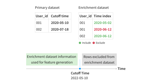
In the primary dataset, the cutoff time for “User_id” 001 is 2020-05-10, so, the recipe will include the row corresponding to 2020-05-02 from the enrichment dataset, but not the row corresponding to 2020-06-12 as it comes after 2020-05-10, the cutoff time. For “User_id” 002, however, the cutoff time is 2020-07-18, so the recipe keeps the row available on 2020-06-12.
Select columns for computation
For each dataset, select the columns that you want to use to compute your features. Note the following :
Original values will also be retrieved for selected columns in the primary dataset or any datasets which the primary dataset has a one-to-one or many-to-one relationship with.
If you used the same dataset more than once in the “Data relationships” tab, the selections will be applied globally for all usage of that dataset.
You may edit the variable types to change the types of transformations performed on the selected column. The next section explains feature transformations in more detail.
Select feature transformations
Choose the transformations that you want to apply to the columns selected in the “Columns for computation” tab. The features differ depending on the variables types of the columns, defined in the “Columns for computation” tab. Two types of transformations exist:
Row-by-row computations
Applied on one row at a time
Performed on all datasets regardless of the relationship types
Run on date & text variable types
Aggregations
Applied across many rows at a time
Performed only on datasets that are on the right side of a one-to-many relationship
Run on general, categorical & numerical variable types
More specifically…
The row-by-row computations consist of :
Date :
Hour: the hour of the day
Day of week
Day of month
Month: the month of the year
Week: the week of the year
Year
Text :
Character count: the number of characters
Word count: the number of spaces in a string + 1
Note
For most databases, the word count first cleans strings to remove consecutive white spaces, tabs and new lines. The SQL databases that do not support REGEX such as SQL Server and Azure Synapse implement a more basic cleaning which keeps tabs, new lines and consecutive spaces (if there are 4 consecutive spaces or more). To improve the accuracy of the word count, you may want to clean your text data in a prepare recipe before using the generate features recipe.
The aggregations consist of :
General :
Count: the count of records
Categorical :
Count distinct: the count of distinct values
Numerical :
Average
Maximum
Minimum
Sum
Output column naming
The recipe derives the output column names from their origin datasets and the transformations. For example, the visual below illustrates how the recipe generates the column name for the count of distinct transaction days:
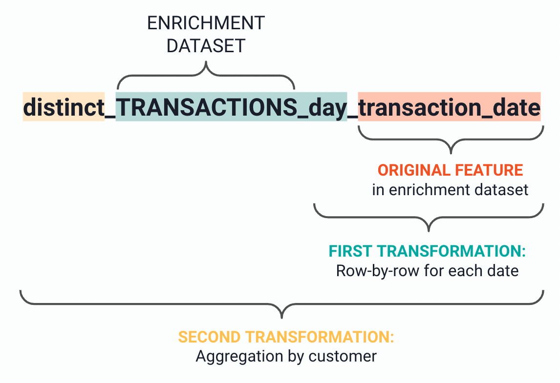
To better explain each computation, the recipe creates column descriptions which help clarify the output features. In the previous example, the recipe describes the column “distinct_TRANSACTIONS_day_date” as follows: “count of distinct values of day of the month of transaction_date for each customer_id in transactions’
Limitations
The generate features recipe only accepts SQL and spark compatible datasets. If Spark is disabled on the Dataiku instance, the input and the output datasets of a recipe must all belong to the same connection.
The recipe does not support partitioned datasets.
The recipe does not support SQL pipelines
Reduce the complexity of the recipe
To reduce the number of generated features, you may :
Decrease the number of relationships.
Create most relationships from the primary dataset instead of the enrichment datasets. If you enrich enrichment datasets, then their enriched version adds up to the primary dataset. As a result, it generates a lot of new features.
Deselect some columns for computation.
Deselect some feature transformations.
The generated features can get quite complex. To generate simpler features, you can :
Avoid using several join conditions. One-to-many relationships use join keys as group keys. So if you select many join keys, the recipe aggregates on multiple columns.
Create most relationships from the primary dataset instead of the enrichment datasets.